Mirrorstoolkit: one-liner analysis tool

library(dplyr)
#> Warning: package 'dplyr' was built under R version 4.4.3
#> 
#> Attaching package: 'dplyr'
#> The following objects are masked from 'package:stats':
#> 
#>     filter, lag
#> The following objects are masked from 'package:base':
#> 
#>     intersect, setdiff, setequal, union
library(readxl)
library(mirrorstoolkit)

Data Preparation

Compute NIH equation 2 for LDL (calc) estimation

compute_nih_ldl functions allows either value or vectorized operation

By value

Simply input the value

mirrorstoolkit::compute_nih_ldl(tchol = 112.9,hdl = 39.9, trig = 151)
#> [1] 47.18626

Vectorized

Use the column name, it uses basic dplyr naming flow. If your column name is not one character string surround it by “`”

df = df %>% dplyr::mutate(
  `LDL (calc) mg/dL` = mirrorstoolkit::compute_nih_ldl(
    tchol = `Chol mg/dL`,
    hdl = `HDL mg/dL`,
    trig = `Trig mg/dL`))

df %>% 
  dplyr::select(
    tidyr::all_of(
      c("Chol mg/dL", 
        "HDL mg/dL",
        "Trig mg/dL", 
        "LDL (calc) mg/dL")
      )) %>% head()
#> # A tibble: 6 × 4
#>   `Chol mg/dL` `HDL mg/dL` `Trig mg/dL` `LDL (calc) mg/dL`
#>          <dbl>       <dbl>        <dbl>              <dbl>
#> 1         113.        39.9          151               47.2
#> 2         189.        76.5          146               87.8
#> 3          92         49.2           82               26.1
#> 4         153.        29.4          315               73.0
#> 5         134.        58.8           83               59.7
#> 6         105.        41.3          145               38.7

Exploratory Data Analysis

Single Group analysis

Normality Inspection

This is a part which I feel is not emphasized enough in our lab practice - we need to determine if a lab evaluation or result result is normally distributed. inspect_distribution() can give a basic visualization about the distribution by

The histogram
The density plot
Shapiro-Wilk test result - please be aware that the null hypothesis is it’s normally distributed, thus if it is significant, it is not normal.

It usually gives a lot of warnings (depends on the completeness and quality of your data for most of the times), I suppressed them here for tidiness, but expose the warnings (omit the last function) are recommended, it will give you useful informations.

Please always be aware that the normality it’s a very subjective decision, always add a huge grab of your own salts from your reading and experience, especially when you have a small sample size. See below, from my perspective:

Albumin, from PMID: 18405401, is generally normal overall.
Calcium is quite normal, which is a bit out of my expectation.
Smoking is actually boolean (binary, 0/1).
LDL, it is on you, you can either treat it as normal or not normal, my experience is it’s generally normal.
wIS often treated as normally distributed on my side.
Lp(a), skewed right for sure

mirrorstoolkit::inspect_distribution(
  data = df, 
  variable = c(
    "Albumin", 
    "Calcium",
    "Smoking",
    "LDL (calc) mg/dL",
    "wIS",
    "Lp(a) (nmol/L)")
  ) %>% base::suppressWarnings()
#> $visualization
#> $`1`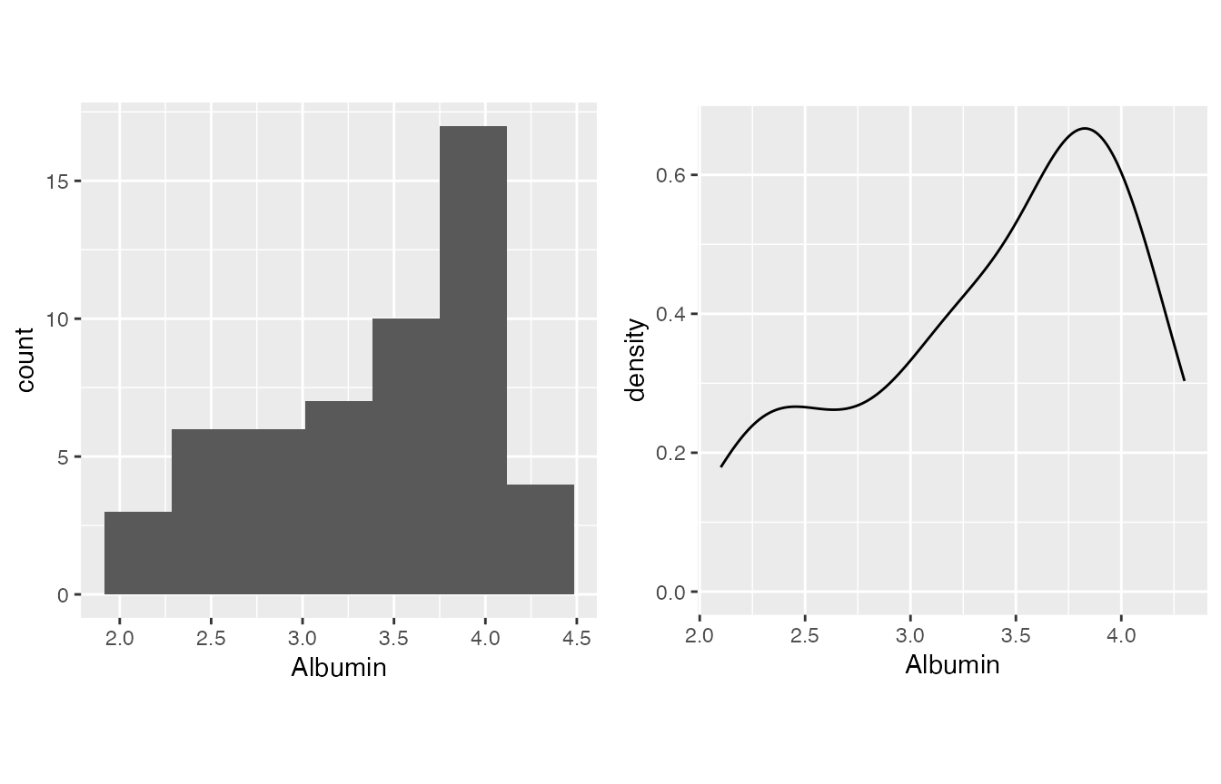

#> 
#> $`2`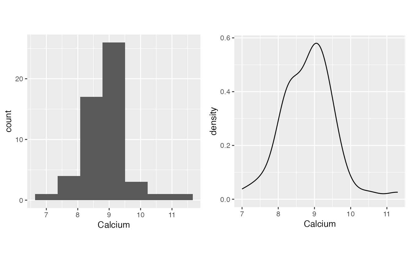

#> 
#> $`3`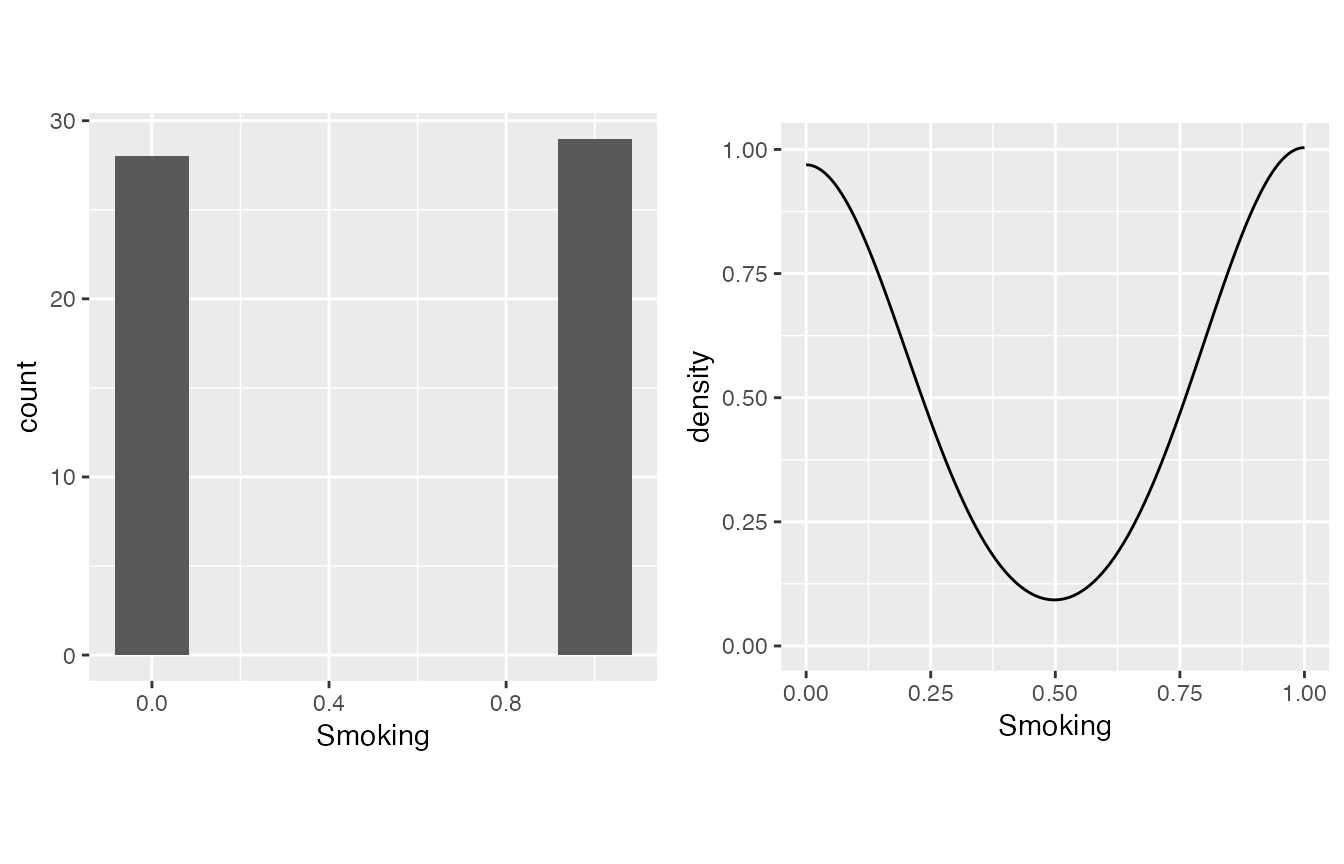

#> 
#> $`4`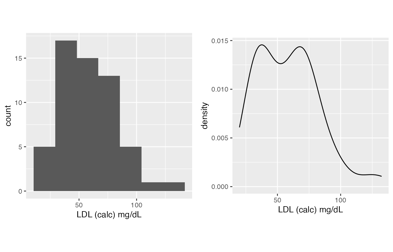

#> 
#> $`5`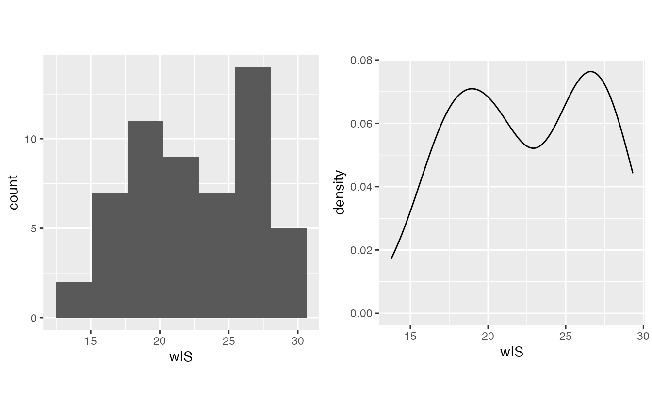

#> 
#> $`6`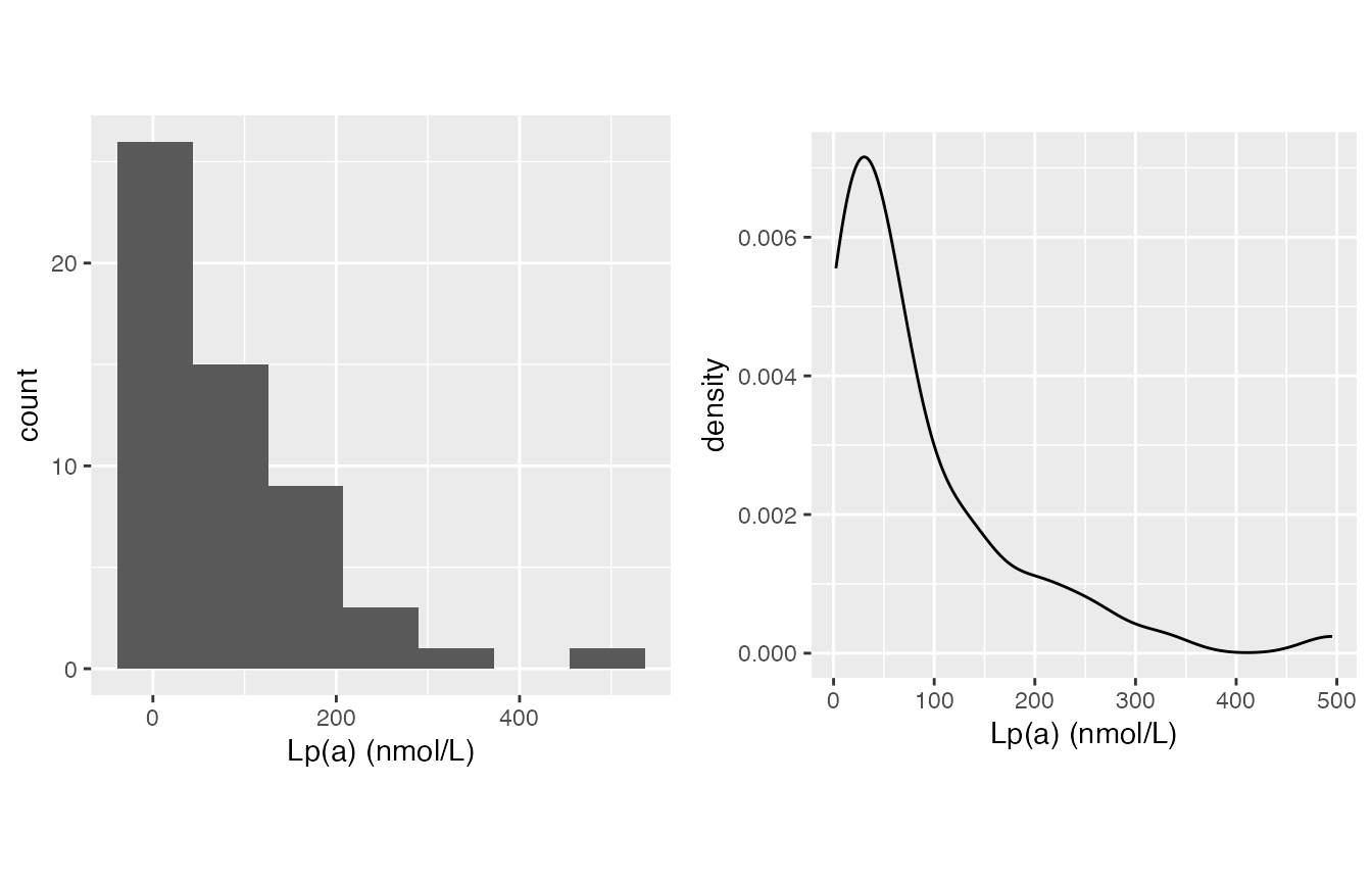

#> 
#> attr(,"class")
#> [1] "list"      "ggarrange"
#> 
#> $`shapiro-wilk_test`
#>           variable      p_value normality
#> 1          Albumin 2.016173e-03     FALSE
#> 2          Calcium 6.699764e-02      TRUE
#> 3 LDL (calc) mg/dL 1.457113e-02     FALSE
#> 4   Lp(a) (nmol/L) 5.255467e-08     FALSE
#> 5          Smoking 1.278103e-10     FALSE
#> 6              wIS 7.879851e-03     FALSE

Characteristic Table

With the result above, you can make your decision and generate a characteristic table.

Boolean (1/0) data should be in boolean_list, the ratio of 1 will be computed
Normally distributed continuous data should be in sd_list, the mean(sd) will be computed
Non-normally distributed continuous data should be in IQR_list, the median(IQR) will be computed

These three lists can be skipped if you don’t have one variable falls into this category.

mirrorstoolkit::characteristic_table_generator(
  data = df,
  boolean_list = c("Smoking"),
  sd_list = c(
    "Calcium", 
    "wIS", 
    "LDL (calc) mg/dL",
    "Albumin"
    ),
  IQR_list = "Lp(a) (nmol/L)",
  order = c(
    "Smoking", 
    "Albumin",
    "Calcium", 
    "LDL (calc) mg/dL",
    "wIS",
    "Lp(a) (nmol/L)")
)
#>                              overall
#> Smoking                29/57(50.88%)
#> Albumin                   3.4 ± 0.63
#> Calcium                  8.83 ± 0.73
#> LDL (calc) mg/dL       58.34 ± 24.31
#> wIS                     22.46 ± 4.45
#> Lp(a) (nmol/L)   46.76(19.66-118.88)

Another implementation can be used here (although I prefer the one above), I don’t know why R original output is not a table for multi-column summary.

Please be aware that this one will run summary() for all columns provided in this table.

mirrorstoolkit::multi_line_summary(
  df[,c(
    "Smoking", 
    "Albumin",
    "Calcium", 
    "LDL (calc) mg/dL",
    "wIS",
    "Lp(a) (nmol/L)")])
#> Warning in (function (..., deparse.level = 1) : number of rows of result is not
#> a multiple of vector length (arg 1)
#>                      Min.  1st Qu.   Median       Mean  3rd Qu.     Max.
#> Smoking           0.00000  0.00000  1.00000  0.5087719   1.0000   1.0000
#> Albumin           2.10000  3.00000  3.60000  3.3981132   3.9000   4.3000
#> Calcium           7.00000  8.30000  8.90000  8.8339623   9.3000  11.3000
#> LDL (calc) mg/dL 19.95264 36.36183 57.88097 58.3391133  72.3185 132.4144
#> wIS              13.76000 18.37000 21.80000 22.4583636  26.3950  29.3200
#> Lp(a) (nmol/L)    2.36000 19.65500 46.76000 82.5434545 118.8850 495.4500
#>                      NA's
#> Smoking           0.00000
#> Albumin           4.00000
#> Calcium           4.00000
#> LDL (calc) mg/dL 19.95264
#> wIS               2.00000
#> Lp(a) (nmol/L)    2.00000

For two groups result

Most of our analysis is based on two groups, e.g. African American vs Caucasians, Study vs control, etc.

Normality Inspection

Add a “by” variable will classify the data. However, I’d suggest keep watching it overall for the distribution. This is simply for completeness in quick inspection.

mirrorstoolkit::inspect_distribution(
  data = df, 
  by = "Race",
  variable = c(
    "Albumin", 
    "Calcium",
    "Smoking",
    "LDL (calc) mg/dL",
    "wIS",
    "Lp(a) (nmol/L)")
  ) %>% base::suppressWarnings()
#> $visualization
#> $`1`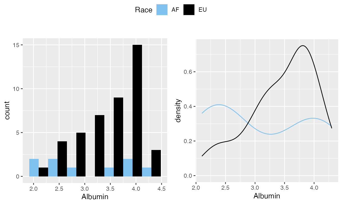

#> 
#> $`2`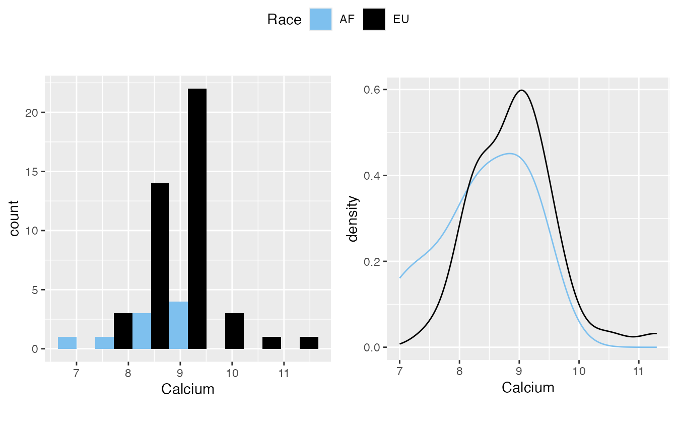

#> 
#> $`3`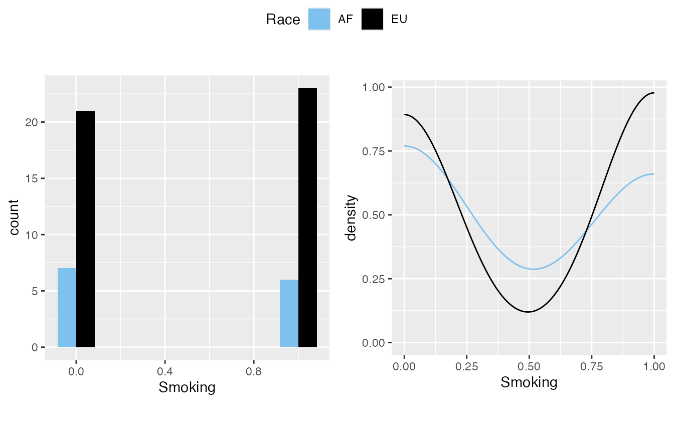

#> 
#> $`4`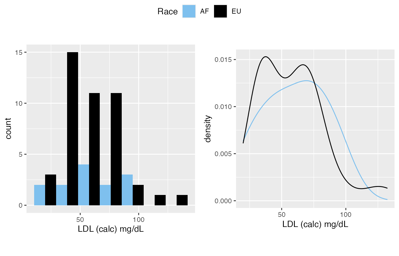

#> 
#> $`5`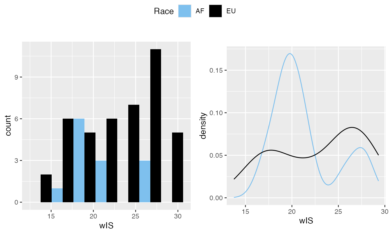

#> 
#> $`6`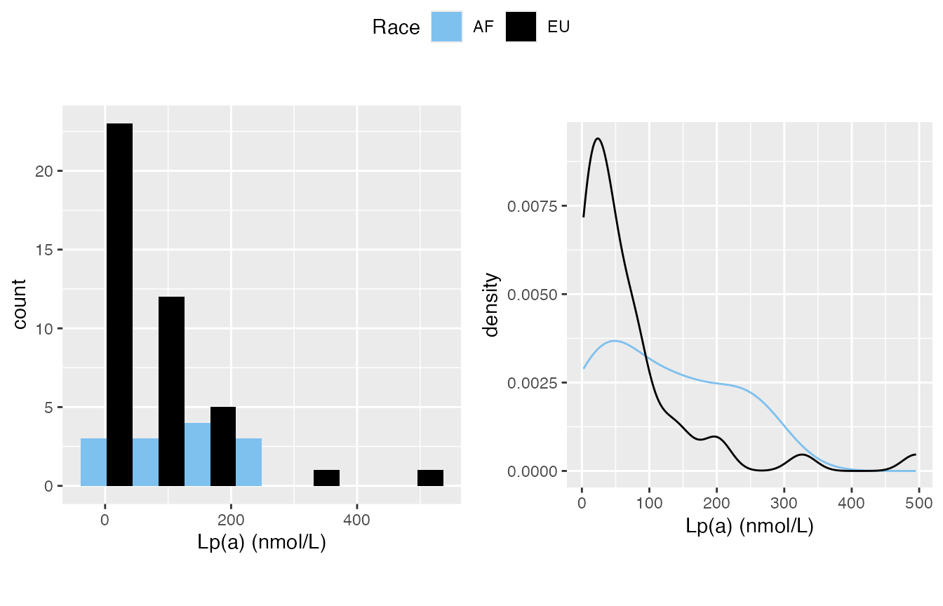

#> 
#> attr(,"class")
#> [1] "list"      "ggarrange"
#> 
#> $`shapiro-wilk_test`
#>           variable      p_value normality             AF             EU
#> 1          Albumin 2.016173e-03     FALSE FALSE(3.3e-02) FALSE(1.9e-02)
#> 2          Calcium 6.699764e-02      TRUE  TRUE(4.9e-01) FALSE(3.0e-02)
#> 3 LDL (calc) mg/dL 1.457113e-02     FALSE  TRUE(9.2e-01) FALSE(3.6e-03)
#> 4   Lp(a) (nmol/L) 5.255467e-08     FALSE  TRUE(1.9e-01) FALSE(1.7e-08)
#> 5          Smoking 1.278103e-10     FALSE FALSE(1.7e-04) FALSE(3.4e-09)
#> 6              wIS 7.879851e-03     FALSE FALSE(4.5e-02) FALSE(6.8e-03)

Characteristic Table

With a “by” provided, it will generate statistics for sub-class, meanwhile a p_value column is provided.

For variables in boolean_list, the p-value is from chi-square test (stats::chisq.test())
For variables in IQR_list, the p-value is from Mann-Whitney U test (Wilcoxon rank-sum test, stats::wilcox.test())
For varaibles in sd_list, the p-value is depending on variable normal_policy
- if normal_policy is “wilcox”(default): it will run Mann-Whitney U test, for the following two reason:
  - Our normal data is often not “that normal”.
  - A sample size of 30 or more is often cited as a general guideline to ensure a normal distribution is a reasonable approximation.
- if normal_policy is “t-test”: it will run Welch’s t-test (stats::t.test(var.equal = FALSE)), which is a more reliable adaptation of Student’s t-test when the two samples have unequal variances and possibly unequal sample sizes

mirrorstoolkit::characteristic_table_generator(
  data = df,
  by = "Race",
  boolean_list = c("Smoking"),
  sd_list = c(
    "Calcium", 
    "wIS", 
    "LDL (calc) mg/dL",
    "Albumin"
    ),
  IQR_list = "Lp(a) (nmol/L)",
  order = c(
    "Smoking", 
    "Albumin",
    "Calcium", 
    "LDL (calc) mg/dL",
    "wIS",
    "Lp(a) (nmol/L)"),
  normal_policy = "t-test"
)
#>                              overall                   AF                 EU
#> Smoking                29/57(50.88%)         6/13(46.15%)      23/44(52.27%)
#> Albumin                   3.4 ± 0.63           3.1 ± 0.88        3.46 ± 0.56
#> Calcium                  8.83 ± 0.73          8.41 ± 0.79         8.92 ± 0.7
#> LDL (calc) mg/dL       58.34 ± 24.31        60.24 ± 24.85      57.78 ± 24.41
#> wIS                     22.46 ± 4.45         21.31 ± 3.52       22.81 ± 4.68
#> Lp(a) (nmol/L)   46.76(19.66-118.88) 127.64(46.92-197.37) 41.08(15.27-79.61)
#>                     p_value
#> Smoking          7.5912e-01
#> Albumin          2.6747e-01
#> Calcium          9.9941e-02
#> LDL (calc) mg/dL 7.5591e-01
#> wIS              2.2530e-01
#> Lp(a) (nmol/L)   4.8697e-02

For 3+ groups result

Normality Inspection

Normality inspection is same as the 2 groups result

Characteristic Table

With a “by” provided, it will generate statistics for sub-class, meanwhile a p_value column is provided.

For variables in boolean_list, the p-value is from chi-square test (stats::chisq.test())
For variables in IQR_list, the p-value is from Kruskal–Wallis test (stats::kruskal.test())
For varaibles in sd_list, the p-value is depending on variable normal_policy
- if normal_policy is “wilcox”(default, I inherited the name from above thus won’t make things too complex): it will run stats::kruskal.test(), for the following two reason:
  - Our normal data is often not “that normal”.
  - A sample size of 30 or more is often cited as a general guideline to ensure a normal distribution is a reasonable approximation.
- if normal_policy is “t-test”: it will run ANOVA(stats::aov())

df = df %>% dplyr::mutate(
  Calciphylaxis_str = Calciphylaxis %>% plyr::mapvalues(c(0,1), c("control", "disease")),
  group = paste(`Race`, `Calciphylaxis_str`, sep = "_"))

df$group %>% table()
#> .
#> AF_control AF_disease EU_control EU_disease 
#>          8          5         22         22

table_1_by_group = mirrorstoolkit::characteristic_table_generator(
  data = df,
  by = "group",
  boolean_list = c("Smoking"),
  sd_list = c(
    "Calcium", 
    "wIS", 
    "LDL (calc) mg/dL",
    "Albumin"
    ),
  IQR_list = "Lp(a) (nmol/L)",
  order = c(
    "Smoking", 
    "Albumin",
    "Calcium", 
    "LDL (calc) mg/dL",
    "wIS",
    "Lp(a) (nmol/L)"),
  normal_policy = "t-test"
)
table_1_by_group
#>                              overall          AF_control          AF_disease
#> Smoking                29/57(50.88%)            4/8(50%)            2/5(40%)
#> Albumin                   3.4 ± 0.63         3.52 ± 0.83         2.76 ± 0.83
#> Calcium                  8.83 ± 0.73          8.7 ± 0.45         8.18 ± 0.97
#> LDL (calc) mg/dL       58.34 ± 24.31       64.04 ± 28.44       54.16 ± 19.04
#> wIS                     22.46 ± 4.45        22.22 ± 3.48         19.85 ± 3.4
#> Lp(a) (nmol/L)   46.76(19.66-118.88) 137.46(43.7-206.76) 55.59(51.67-129.45)
#>                          EU_control        EU_disease    p_value
#> Smoking               12/22(54.55%)        11/22(50%) 9.8051e-01
#> Albumin                  3.82 ± 0.3        3.1 ± 0.54 2.8352e-05
#> Calcium                 8.79 ± 0.54       9.05 ± 0.82 1.0060e-01
#> LDL (calc) mg/dL      56.18 ± 17.64     59.38 ± 30.07 8.5607e-01
#> wIS                    22.98 ± 4.51      22.65 ± 4.96 5.7002e-01
#> Lp(a) (nmol/L)   33.85(18.76-87.43) 43.4(14.11-75.14) 2.0291e-01

The output illutrated the p-value as literal string for I need to keep the format for paper use… To filter the p-value you can do this

table_1_by_group %>% 
  dplyr::mutate(p_value = p_value %>% as.numeric()) %>% 
  dplyr::filter(p_value < 0.05)
#>            overall  AF_control  AF_disease EU_control EU_disease    p_value
#> Albumin 3.4 ± 0.63 3.52 ± 0.83 2.76 ± 0.83 3.82 ± 0.3 3.1 ± 0.54 2.8352e-05

Pairwise test

Please always be aware that for 3+ group test, one p-value is not sufficient to claim too much stuff. Multi-class chi-square/Kruskal-Wallis/ANOVA only told you “some group is different from the other”

Boolean Variables

Pairwise comparisons between pairs of proportions (stats::pairwise.prop.test) used here, a filled barchart used in the visualization.

When the pairwise test is throwing “Warning: Chi-squared approximation may be incorrect” means that one or more of your table’s expected cell counts are too small for the Chi-squared test to be reliable, typically when they are less than 5. This violates the test’s assumptions, and you should address it by either increasing sample size, combining categories, or using an alternative like Fisher’s exact test or a simulated p-value.

If it’s labelled significant, it can be a good support to your claim.
If it’s not labelled as significant, it doesn’t always mean that they are not different, it’s simply stats::pairwise.prop.test cannot handle it. Be bold to make your choice.

Some settings, I grabbed a setting from the air for the illustration:

adjustment_method The choice of this variable is from here. “fdr” (Benjamini-Hochberg FDR correction) by default thus you can often skip it.
p_threshold will affect the filtering from first to second table, the significant result will be labelled on the top of the figure, 0.05 by default
variable can take one or more variables.

pairwise_boolean = mirrorstoolkit::pairwise_boolean_report(
  data = df, 
  variable = c("antiplatelet_group", "statin_group"), 
  by = "group",
  adjustment_method = "none",
  p_threshold = 0.3)
#> Warning in prop.test(x[c(i, j)], n[c(i, j)], ...): Chi-squared approximation
#> may be incorrect
#> Warning in prop.test(x[c(i, j)], n[c(i, j)], ...): Chi-squared approximation
#> may be incorrect
#> Warning in prop.test(x[c(i, j)], n[c(i, j)], ...): Chi-squared approximation
#> may be incorrect
#> Warning in prop.test(x[c(i, j)], n[c(i, j)], ...): Chi-squared approximation
#> may be incorrect
#> Warning in prop.test(x[c(i, j)], n[c(i, j)], ...): Chi-squared approximation
#> may be incorrect
#> Warning in prop.test(x[c(i, j)], n[c(i, j)], ...): Chi-squared approximation
#> may be incorrect
#> Warning in prop.test(x[c(i, j)], n[c(i, j)], ...): Chi-squared approximation
#> may be incorrect
#> Warning in prop.test(x[c(i, j)], n[c(i, j)], ...): Chi-squared approximation
#> may be incorrect
#> Warning in prop.test(x[c(i, j)], n[c(i, j)], ...): Chi-squared approximation
#> may be incorrect
#> Warning in prop.test(x[c(i, j)], n[c(i, j)], ...): Chi-squared approximation
#> may be incorrect
#> Warning in ggsignif::geom_signif(data = annotation_significant,
#> ggplot2::aes(xmin = group1, : Ignoring unknown aesthetics: xmin,
#> xmax, annotations, and y_position

pairwise_boolean$result
#> # A tibble: 12 × 4
#>    variable_name      group1     group2     p_value
#>    <chr>              <chr>      <chr>        <dbl>
#>  1 antiplatelet_group AF_disease AF_control   0.396
#>  2 antiplatelet_group EU_control AF_control   1.00 
#>  3 antiplatelet_group EU_control AF_disease   0.357
#>  4 antiplatelet_group EU_disease AF_control   1    
#>  5 antiplatelet_group EU_disease AF_disease   0.281
#>  6 antiplatelet_group EU_disease EU_control   0.931
#>  7 statin_group       AF_disease AF_control   1    
#>  8 statin_group       EU_control AF_control   1    
#>  9 statin_group       EU_control AF_disease   1    
#> 10 statin_group       EU_disease AF_control   0.907
#> 11 statin_group       EU_disease AF_disease   1    
#> 12 statin_group       EU_disease EU_control   0.803

pairwise_boolean$significant_result
#> # A tibble: 1 × 4
#>   variable_name      group1     group2     p_value
#>   <chr>              <chr>      <chr>        <dbl>
#> 1 antiplatelet_group EU_disease AF_disease    0.28

pairwise_boolean$plot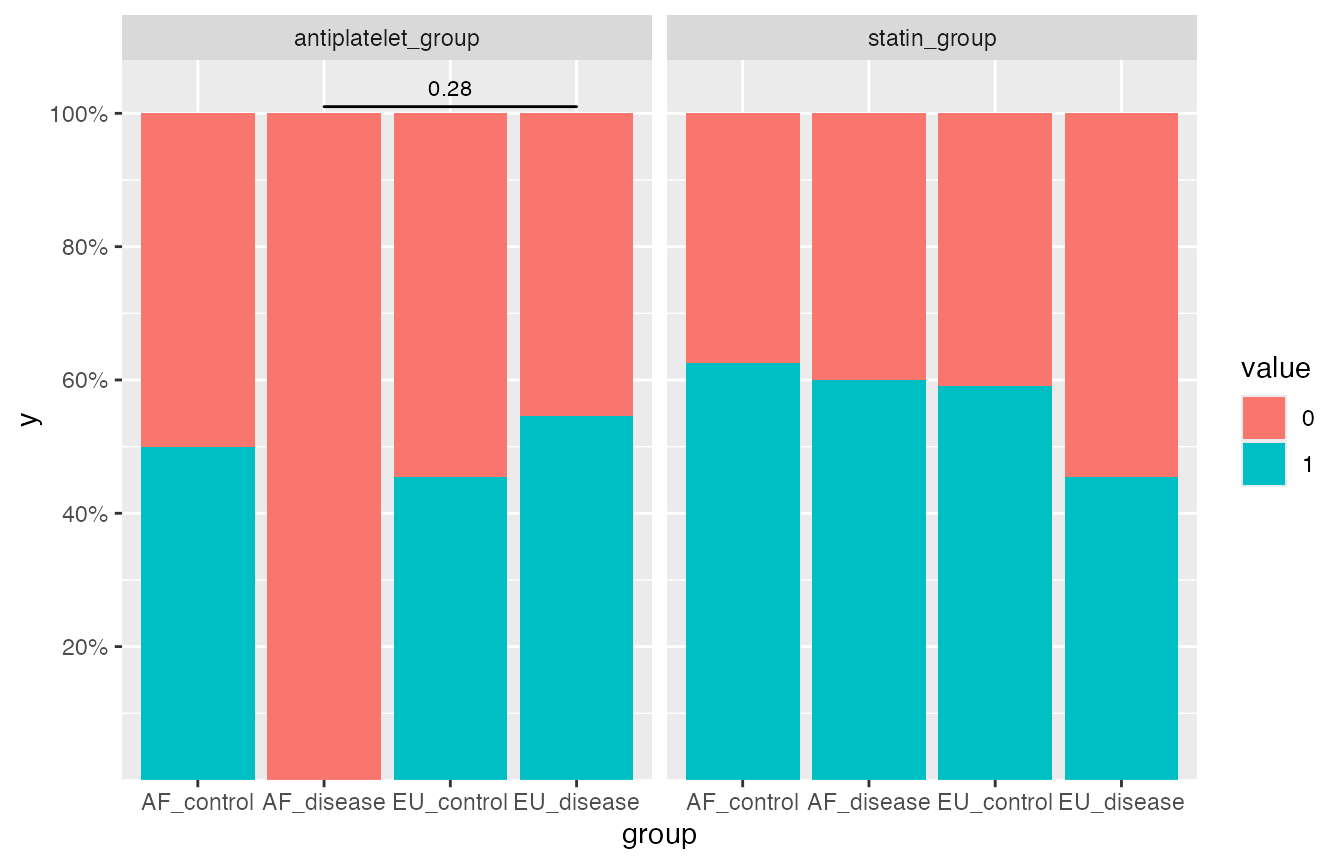

Not Normally Distributed Continuous Variables

Pairwise Mann-Whiteney U-test (stats::pairwise.wilcox.test) used here, boxplot for illustration.

If you are not confident with the normality or the sample size, use this one.

Please be aware of a toxic chemical reaction here:

Mann-Whiteney U test is based on the rank of the sample
Boxplot can drop some outliers out.

Thus this report is very visually misleading with extremely small sample size, e.g. AF_disease group only have 5 samples and 1 outliers makes it not significantly different from the other

df$`Lp(a) (nmol/L)`
#>  [1] 204.60   7.77  30.60     NA  18.76  86.02  33.85   6.33  31.30  33.85
#> [11]  38.89  58.27   9.88  29.37 252.60  34.02  10.87  46.92 147.29 127.64
#> [21] 234.93  13.59 197.37  87.43 495.45   3.97 125.88 156.62  74.34 195.71
#> [31]  20.55  78.89  43.26  75.14 129.45   3.37  55.59   4.65   8.23  79.85
#> [41] 111.89  43.40  46.76  51.67  33.39   4.65  20.83  44.61  14.11  55.33
#> [51] 326.37  74.65   2.36 273.65     NA 139.47   3.65

pairwise_wilcox = mirrorstoolkit::pairwise_wilcox_report(
  data = df, 
  variable = "Lp(a) (nmol/L)", 
  by = "group",
  p_threshold = 0.30
)
#> Warning in ggsignif::geom_signif(data = annotation_significant,
#> ggplot2::aes(xmin = group1, : Ignoring unknown aesthetics: xmin,
#> xmax, annotations, and y_position

pairwise_wilcox$result
#> # A tibble: 6 × 4
#>   variable_name  group1     group2     p_value
#>   <chr>          <chr>      <chr>        <dbl>
#> 1 Lp(a) (nmol/L) AF_disease AF_control   0.826
#> 2 Lp(a) (nmol/L) EU_control AF_control   0.250
#> 3 Lp(a) (nmol/L) EU_control AF_disease   0.738
#> 4 Lp(a) (nmol/L) EU_disease AF_control   0.250
#> 5 Lp(a) (nmol/L) EU_disease AF_disease   0.738
#> 6 Lp(a) (nmol/L) EU_disease EU_control   0.738

pairwise_wilcox$significant_result
#> # A tibble: 2 × 4
#>   variable_name  group1     group2     p_value
#>   <chr>          <chr>      <chr>        <dbl>
#> 1 Lp(a) (nmol/L) EU_control AF_control    0.25
#> 2 Lp(a) (nmol/L) EU_disease AF_control    0.25

pairwise_wilcox$plot
#> Warning: Removed 2 rows containing non-finite outside the scale range
#> (`stat_boxplot()`).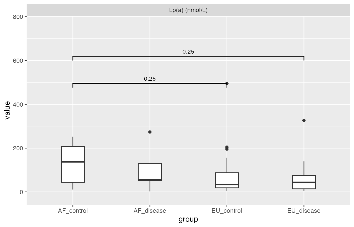

Normally Distributed Continuous Variables

Pairwise t-test (stats::pairwise.t.test) used here, barchart for mean with errorbar (1 sd, not 95% CI) for illustration.

Still, if you are not confident with the normality or the sample size, use the one for not normally distributed variable above.

pairwise_t_test = mirrorstoolkit::pairwise_t_test_report(
  data = df, 
  variable = c("Calcium","Albumin"), 
  by = "group",
  p_threshold = 0.15
)
#> Warning in ggsignif::geom_signif(data = annotation_significant,
#> ggplot2::aes(xmin = group1, : Ignoring unknown aesthetics: xmin,
#> xmax, annotations, and y_position

pairwise_t_test$result
#> # A tibble: 12 × 4
#>    variable_name group1     group2      p_value
#>    <chr>         <chr>      <chr>         <dbl>
#>  1 Albumin       AF_disease AF_control 0.0617  
#>  2 Albumin       EU_control AF_control 0.298   
#>  3 Albumin       EU_control AF_disease 0.000379
#>  4 Albumin       EU_disease AF_control 0.201   
#>  5 Albumin       EU_disease AF_disease 0.225   
#>  6 Albumin       EU_disease EU_control 0.000156
#>  7 Calcium       AF_disease AF_control 0.416   
#>  8 Calcium       EU_control AF_control 0.814   
#>  9 Calcium       EU_control AF_disease 0.261   
#> 10 Calcium       EU_disease AF_control 0.439   
#> 11 Calcium       EU_disease AF_disease 0.0977  
#> 12 Calcium       EU_disease EU_control 0.416

pairwise_t_test$significant_result
#> # A tibble: 4 × 4
#>   variable_name group1     group2     p_value
#>   <chr>         <chr>      <chr>        <dbl>
#> 1 Albumin       AF_disease AF_control 0.062  
#> 2 Albumin       EU_control AF_disease 0.00038
#> 3 Albumin       EU_disease EU_control 0.00016
#> 4 Calcium       EU_disease AF_disease 0.098

pairwise_t_test$plot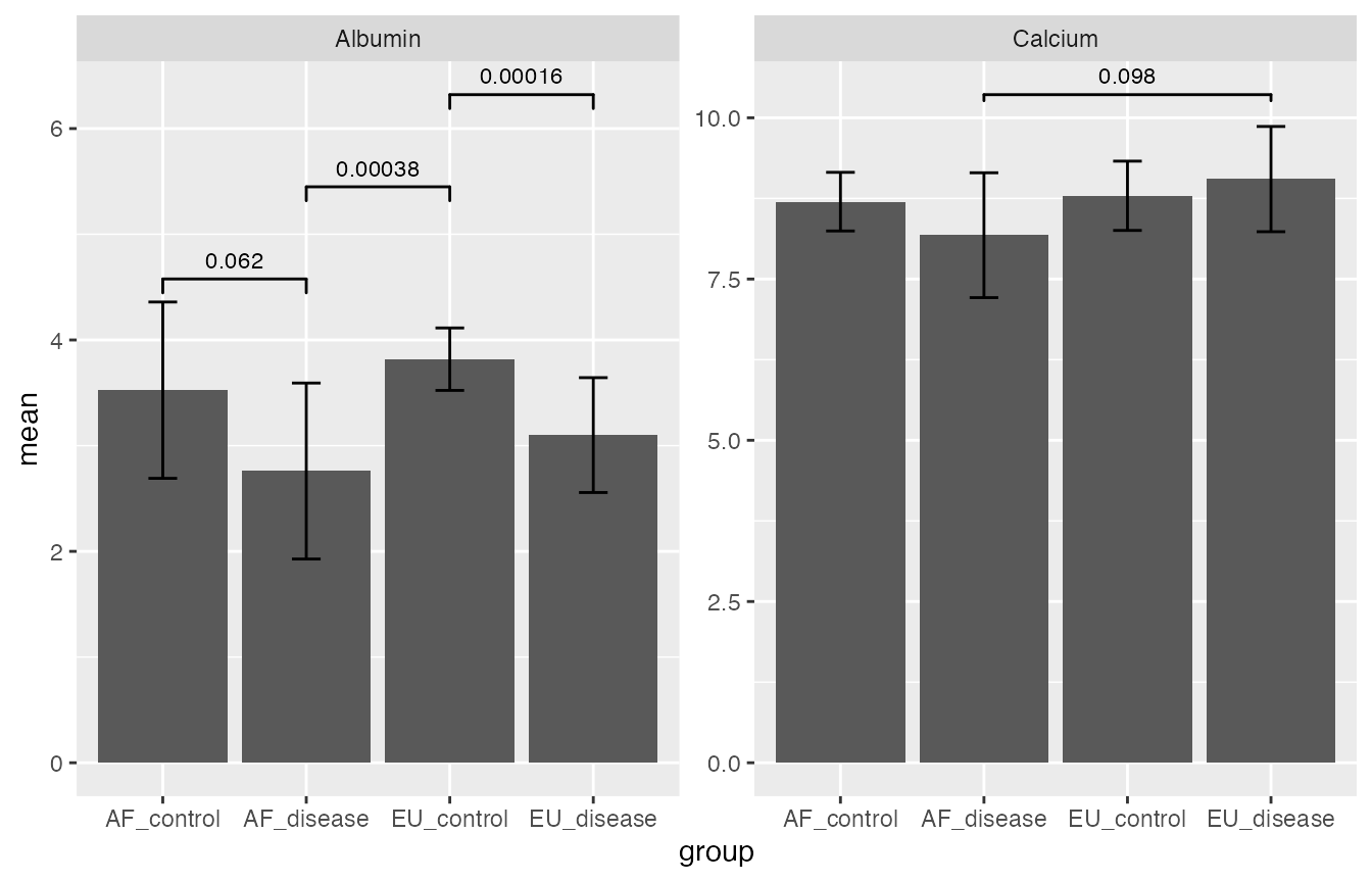

If you only want the first table in supplemental data, you can run the one below as well. Replace “report” to “table” in the function name and remove the p_threshold if you have. This function is internally called in mirrorstoolkit::pairwise_t_test_report, so do the other two.

mirrorstoolkit::pairwise_t_test_table(
  data = df, 
  variable = "Calcium", 
  by = "group"
)
#> # A tibble: 6 × 4
#>   variable_name group1     group2     p_value
#>   <chr>         <chr>      <chr>        <dbl>
#> 1 Calcium       AF_disease AF_control  0.416 
#> 2 Calcium       EU_control AF_control  0.814 
#> 3 Calcium       EU_control AF_disease  0.261 
#> 4 Calcium       EU_disease AF_control  0.439 
#> 5 Calcium       EU_disease AF_disease  0.0977
#> 6 Calcium       EU_disease EU_control  0.416

Correlation matrix

We provide two functions for correlation matrix analysis.

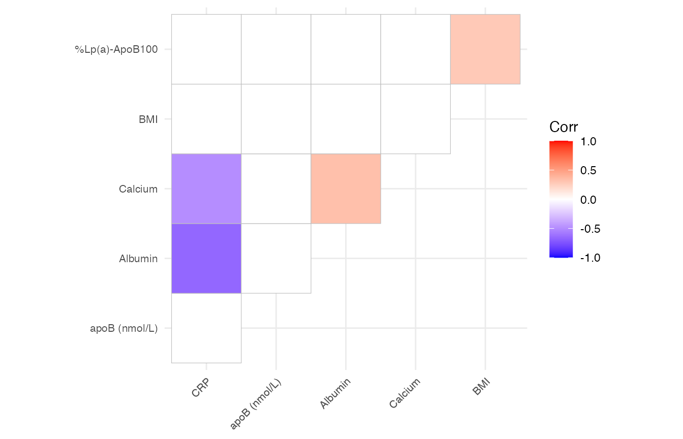
To visualize the correlation matrix

mirrorstoolkit::correlation_matrix_plot will return a ggplot2 instance, sharing a similar argument setting:

variable is optional, if not provided, will use all the columns provided in data. However, as a fool-proofing operation, providing the variable column is a good sanity check as the function will internally enforces all the value in your data table to numeric.
font_size is 5 by default for all labels.
please be aware that the order is reordered by hierarchical clustering for better cluster illustration

mirrorstoolkit::correlation_matrix_plot(
  data = df,
  variable = c("BMI", "Albumin", "Calcium", "CRP", "apoB (nmol/L)","%Lp(a)-ApoB100"),
  font_size = 8
)
#> Warning: `aes_string()` was deprecated in ggplot2 3.0.0.
#> ℹ Please use tidy evaluation idioms with `aes()`.
#> ℹ See also `vignette("ggplot2-in-packages")` for more information.
#> ℹ The deprecated feature was likely used in the ggcorrplot package.
#>   Please report the issue at <https://github.com/kassambara/ggcorrplot/issues>.
#> This warning is displayed once per session.
#> Call `lifecycle::last_lifecycle_warnings()` to see where this warning was
#> generated.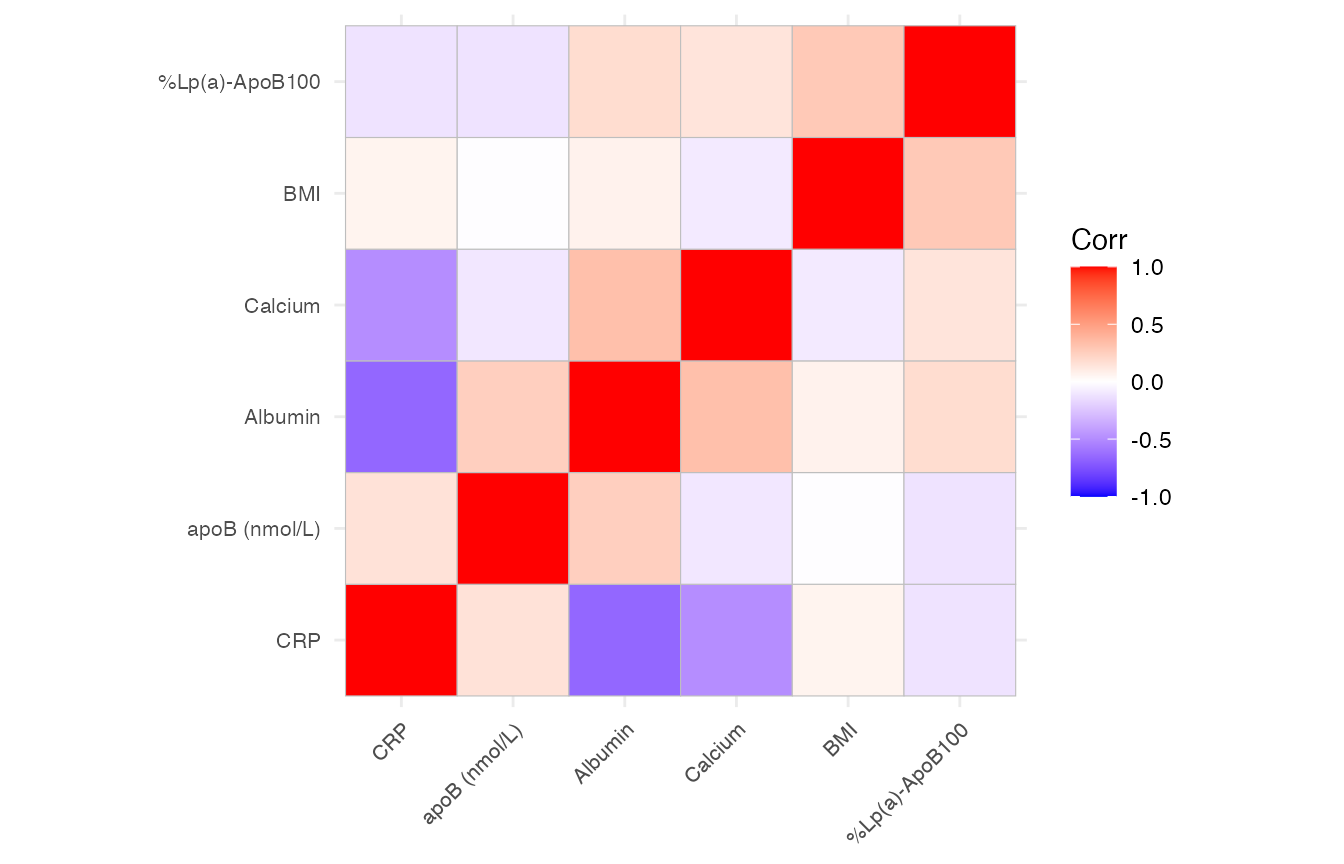

This function also provide a filter operation by the p-value as long as the p_threshold is specified. see below (I changed the way inputting column here for illustration purpose, it doesn’t matter):

mirrorstoolkit::correlation_matrix_plot(
  data = df %>% dplyr::select(
    tidyr::all_of(c("BMI", "Albumin", "Calcium", "CRP", "apoB (nmol/L)","%Lp(a)-ApoB100"))
    ),
  font_size = 8,
  p_threshold = 0.05
)

To further deal with the correlation matrix

For potential multi-omics studies in the future, I left an function here outputting the matrix as data.frame format, which removed all the redundant columns. It has a p_threshold option same as above but I don’t think it’s necessary here.

mirrorstoolkit::correlation_matrix_dataframe(
  data = df,
  variable = c("BMI", "Albumin", "Calcium", "CRP", "apoB (nmol/L)","%Lp(a)-ApoB100")
)
#>              row         column        corr      p_value
#> 1            BMI        Albumin  0.07246750 6.096735e-01
#> 2            BMI        Calcium -0.09116465 5.203815e-01
#> 3        Albumin        Calcium  0.33290055 1.486389e-02
#> 4            BMI            CRP  0.06434398 7.309315e-01
#> 5        Albumin            CRP -0.66165518 3.729085e-05
#> 6        Calcium            CRP -0.48625030 4.776512e-03
#> 7            BMI  apoB (nmol/L) -0.00519316 9.696990e-01
#> 8        Albumin  apoB (nmol/L)  0.25441832 6.600239e-02
#> 9        Calcium  apoB (nmol/L) -0.10436060 4.570736e-01
#> 10           CRP  apoB (nmol/L)  0.15435436 3.989530e-01
#> 11           BMI %Lp(a)-ApoB100  0.27960245 4.059818e-02
#> 12       Albumin %Lp(a)-ApoB100  0.17946329 2.076293e-01
#> 13       Calcium %Lp(a)-ApoB100  0.14327436 3.158588e-01
#> 14           CRP %Lp(a)-ApoB100 -0.11916085 5.231636e-01
#> 15 apoB (nmol/L) %Lp(a)-ApoB100 -0.12428106 3.659771e-01

Composition Component Trends

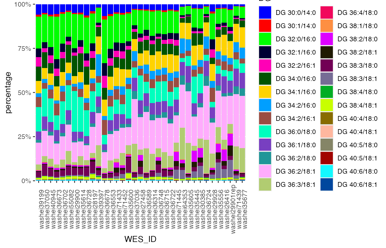
For the illustration of trends of a composition with a set of components

lipidomic_samples %>% head(3)
#>        WES_ID Lp(a) (nmol/L) DG 30:0/14:0 DG 30:1/14:0 DG 32:0/16:0
#> 1 washei26416          157.0 0.0008071535 0.0001372855  0.003098725
#> 2 washei27458           37.1 0.0009333268 0.0002105400  0.004237114
#> 3 washei28197           15.0 0.0032868436 0.0010452749  0.013764988
#>   DG 32:1/16:0 DG 32:2/16:1 DG 34:0/16:0 DG 34:1/16:0 DG 34:2/16:0 DG 34:2/16:1
#> 1 0.0006956733 0.0002478549  0.001698103  0.004516096 0.0013578084  0.001842253
#> 2 0.0007368318 0.0007199269  0.002174789  0.002236245 0.0005861636  0.001207711
#> 3 0.0036933192 0.0031672078  0.005407289  0.004072219 0.0021591445  0.003816118
#>   DG 36:0/18:0 DG 36:1/18:0 DG 36:2/18:0 DG 36:2/18:1 DG 36:3/18:1 DG 36:4/18:0
#> 1  0.001415583  0.003683802 0.0007110398  0.009479445 0.0020066608 9.143163e-06
#> 2  0.004551087  0.002515179 0.0005592532  0.005935862 0.0009731812 2.037506e-05
#> 3  0.009499735  0.005311344 0.0016281908  0.012059293 0.0022217465 0.000000e+00
#>   DG 38:1/18:0 DG 38:2/18:0 DG 38:2/18:1 DG 38:3/18:0 DG 38:3/18:1 DG 38:4/18:0
#> 1 0.0001244584 0.0025175506 0.0009816070 0.0007872274 0.0019228689 4.408206e-05
#> 2 0.0000000000 0.0010531250 0.0011219876 0.0013524833 0.0004459673 4.037663e-05
#> 3 0.0002654990 0.0006729207 0.0008393582 0.0053460809 0.0004614999 1.576657e-04
#>   DG 38:4/18:1 DG 40:4/18:0 DG 40:4/18:1 DG 40:5/18:0 DG 40:5/18:1 DG 40:6/18:0
#> 1 0.0003366250 1.112712e-05 1.190158e-05 4.217323e-05 1.682002e-05 9.500192e-05
#> 2 0.0003986452 2.709289e-05 1.349291e-05 5.475041e-06 1.950699e-05 1.778880e-04
#> 3 0.0018140866 8.260741e-05 9.626816e-05 2.173361e-04 6.999751e-05 5.937550e-04
#>   DG 40:6/18:1
#> 1 7.053647e-05
#> 2 5.693585e-05
#> 3 1.035781e-04

You can either specify the column you want by variable = c(“col1”, “col2”, “col3”) if you need, but most of the times it will be quite lengthy. If it is not specified, it will use all the columns not mentioned in the table.

mirrorstoolkit::trend_bar_chart(
  data = lipidomic_samples,
  id = "WES_ID",
  by = "Lp(a) (nmol/L)",
  legend_title = "DG"
)

Association Studies

For those you are interested, you might want to log them if you think they are not normally distributed:

df = df %>% dplyr::mutate(
  LDL = `LDL (calc) mg/dL`,
  lpa_logged = `Lp(a) (nmol/L)` %>% base::log2(),
)

OLS_wrapper and logistic_wrapper() can deal with most of the association analysis we need. In most of our tasks, we can specify the follow 2 or 3 lists as global settings used repetitively.

# The adjustment variable you need
adjustments = c(
  "Age", 
  "Gender", 
  "AF", 
  "BMI",
  "Smoking",
  "antiplatelet_group", 
  "anticoagulant_group", 
  "statin_group"
  )
# The variable you are interested in
variable_list = c(
  "Albumin",
  "Calcium",
  "LDL",
  "wIS", 
  "lpa_logged")
# In case the column name is not what you want in the output 
variable_list_formal = c(
  "Albumin",
  "Calcium",
  "LDL(calc) mg/dL",
  "wIS",
  "Lp(a) nmol/L, 2-logged"
  )

Logistics regression

The wrapper is runing in the following way:

For each column name mentioned in variable_list, let’s call it variable_i
- Grab the columns mentioned in variable_i, adjustments, and response from data. If variable_i is in adjustments, will remove the duplicates
- Logistic regression response $\sim$ variable_i + adjustment + 1
- Seek the effect size and coefficient of variable_i, compute the odd ratio by exp(effect size)
Collect all the data

What you need to specify is:

data, your dataframe
response, which the column name of your target (y)
adjustments, you adjustment list defined above
by, if you want to categorize the data
variable_of_interest, your variable list
variable_of_interest_formal_name, the variable name list in the data

mirrorstoolkit::logistic_wrapper(
  data = df, 
  response = "Calciphylaxis",
  adjustments = adjustments,
  variable_of_interest = variable_list,
  variable_of_interest_formal_name = variable_list_formal
  )
#>                         Effect Size   Odd Ratio    P-value
#> Albumin                -5.170826684 0.005679871 0.00327561
#> Calcium                 0.833885757 2.302247357 0.11224877
#> LDL(calc) mg/dL         0.006642994 1.006665108 0.61218217
#> wIS                     0.003948747 1.003956554 0.95723792
#> Lp(a) nmol/L, 2-logged  0.014135081 1.014235454 0.94323132

mirrorstoolkit::logistic_wrapper(
  data = df, 
  response = "Calciphylaxis",
  adjustments = adjustments,
  variable_of_interest = variable_list,
  variable_of_interest_formal_name = variable_list_formal,
  with_power = TRUE,
  variable_distribution = c("normal", "normal", "normal", "normal", "normal")
  )
#> +--------------------------------------------------+
#> |                POWER CALCULATION                 |
#> +--------------------------------------------------+
#> 
#> Logistic Regression Coefficient (Wald's Z-Test)
#> 
#>   Method          : Demidenko (Variance Corrected)
#>   Predictor Dist. : Normal
#> 
#> ---------------------------------------------------
#> Hypotheses
#> ---------------------------------------------------
#>   H0 (Null Claim) : Odds Ratio = 1
#>   H1 (Alt. Claim) : Odds Ratio != 1
#> 
#> ---------------------------------------------------
#> Results
#> ---------------------------------------------------
#>   Sample Size          = 52
#>   Type 1 Error (alpha) = 0.050
#>   Type 2 Error (beta)  = 0.970
#>   Statistical Power    = 0.03  <<
#> 
#> +--------------------------------------------------+
#> |             SAMPLE SIZE CALCULATION              |
#> +--------------------------------------------------+
#> 
#> Logistic Regression Coefficient (Wald's Z-Test)
#> 
#>   Method          : Demidenko (Variance Corrected)
#>   Predictor Dist. : Normal
#> 
#> ---------------------------------------------------
#> Hypotheses
#> ---------------------------------------------------
#>   H0 (Null Claim) : Odds Ratio = 1
#>   H1 (Alt. Claim) : Odds Ratio != 1
#> 
#> ---------------------------------------------------
#> Results
#> ---------------------------------------------------
#>   Sample Size          = 243311  <<
#>   Type 1 Error (alpha) = 0.050
#>   Type 2 Error (beta)  = 0.200
#>   Statistical Power    = 0.8
#> 
#> +--------------------------------------------------+
#> |                POWER CALCULATION                 |
#> +--------------------------------------------------+
#> 
#> Logistic Regression Coefficient (Wald's Z-Test)
#> 
#>   Method          : Demidenko (Variance Corrected)
#>   Predictor Dist. : Normal
#> 
#> ---------------------------------------------------
#> Hypotheses
#> ---------------------------------------------------
#>   H0 (Null Claim) : Odds Ratio = 1
#>   H1 (Alt. Claim) : Odds Ratio != 1
#> 
#> ---------------------------------------------------
#> Results
#> ---------------------------------------------------
#>   Sample Size          = 52
#>   Type 1 Error (alpha) = 0.050
#>   Type 2 Error (beta)  = 0.948
#>   Statistical Power    = 0.052  <<
#> 
#> +--------------------------------------------------+
#> |             SAMPLE SIZE CALCULATION              |
#> +--------------------------------------------------+
#> 
#> Logistic Regression Coefficient (Wald's Z-Test)
#> 
#>   Method          : Demidenko (Variance Corrected)
#>   Predictor Dist. : Normal
#> 
#> ---------------------------------------------------
#> Hypotheses
#> ---------------------------------------------------
#>   H0 (Null Claim) : Odds Ratio = 1
#>   H1 (Alt. Claim) : Odds Ratio != 1
#> 
#> ---------------------------------------------------
#> Results
#> ---------------------------------------------------
#>   Sample Size          = 26460  <<
#>   Type 1 Error (alpha) = 0.050
#>   Type 2 Error (beta)  = 0.200
#>   Statistical Power    = 0.8
#> 
#> +--------------------------------------------------+
#> |                POWER CALCULATION                 |
#> +--------------------------------------------------+
#> 
#> Logistic Regression Coefficient (Wald's Z-Test)
#> 
#>   Method          : Demidenko (Variance Corrected)
#>   Predictor Dist. : Normal
#> 
#> ---------------------------------------------------
#> Hypotheses
#> ---------------------------------------------------
#>   H0 (Null Claim) : Odds Ratio = 1
#>   H1 (Alt. Claim) : Odds Ratio != 1
#> 
#> ---------------------------------------------------
#> Results
#> ---------------------------------------------------
#>   Sample Size          = 56
#>   Type 1 Error (alpha) = 0.050
#>   Type 2 Error (beta)  = 0.911
#>   Statistical Power    = 0.089  <<
#> 
#> +--------------------------------------------------+
#> |             SAMPLE SIZE CALCULATION              |
#> +--------------------------------------------------+
#> 
#> Logistic Regression Coefficient (Wald's Z-Test)
#> 
#>   Method          : Demidenko (Variance Corrected)
#>   Predictor Dist. : Normal
#> 
#> ---------------------------------------------------
#> Hypotheses
#> ---------------------------------------------------
#>   H0 (Null Claim) : Odds Ratio = 1
#>   H1 (Alt. Claim) : Odds Ratio != 1
#> 
#> ---------------------------------------------------
#> Results
#> ---------------------------------------------------
#>   Sample Size          = 1244  <<
#>   Type 1 Error (alpha) = 0.050
#>   Type 2 Error (beta)  = 0.200
#>   Statistical Power    = 0.8
#> 
#> +--------------------------------------------------+
#> |                POWER CALCULATION                 |
#> +--------------------------------------------------+
#> 
#> Logistic Regression Coefficient (Wald's Z-Test)
#> 
#>   Method          : Demidenko (Variance Corrected)
#>   Predictor Dist. : Normal
#> 
#> ---------------------------------------------------
#> Hypotheses
#> ---------------------------------------------------
#>   H0 (Null Claim) : Odds Ratio = 1
#>   H1 (Alt. Claim) : Odds Ratio != 1
#> 
#> ---------------------------------------------------
#> Results
#> ---------------------------------------------------
#>   Sample Size          = 54
#>   Type 1 Error (alpha) = 0.050
#>   Type 2 Error (beta)  = 0.950
#>   Statistical Power    = 0.05  <<
#> 
#> +--------------------------------------------------+
#> |             SAMPLE SIZE CALCULATION              |
#> +--------------------------------------------------+
#> 
#> Logistic Regression Coefficient (Wald's Z-Test)
#> 
#>   Method          : Demidenko (Variance Corrected)
#>   Predictor Dist. : Normal
#> 
#> ---------------------------------------------------
#> Hypotheses
#> ---------------------------------------------------
#>   H0 (Null Claim) : Odds Ratio = 1
#>   H1 (Alt. Claim) : Odds Ratio != 1
#> 
#> ---------------------------------------------------
#> Results
#> ---------------------------------------------------
#>   Sample Size          = 101680  <<
#>   Type 1 Error (alpha) = 0.050
#>   Type 2 Error (beta)  = 0.200
#>   Statistical Power    = 0.8
#> 
#> +--------------------------------------------------+
#> |                POWER CALCULATION                 |
#> +--------------------------------------------------+
#> 
#> Logistic Regression Coefficient (Wald's Z-Test)
#> 
#>   Method          : Demidenko (Variance Corrected)
#>   Predictor Dist. : Normal
#> 
#> ---------------------------------------------------
#> Hypotheses
#> ---------------------------------------------------
#>   H0 (Null Claim) : Odds Ratio = 1
#>   H1 (Alt. Claim) : Odds Ratio != 1
#> 
#> ---------------------------------------------------
#> Results
#> ---------------------------------------------------
#>   Sample Size          = 54
#>   Type 1 Error (alpha) = 0.050
#>   Type 2 Error (beta)  = 0.949
#>   Statistical Power    = 0.051  <<
#> 
#> +--------------------------------------------------+
#> |             SAMPLE SIZE CALCULATION              |
#> +--------------------------------------------------+
#> 
#> Logistic Regression Coefficient (Wald's Z-Test)
#> 
#>   Method          : Demidenko (Variance Corrected)
#>   Predictor Dist. : Normal
#> 
#> ---------------------------------------------------
#> Hypotheses
#> ---------------------------------------------------
#>   H0 (Null Claim) : Odds Ratio = 1
#>   H1 (Alt. Claim) : Odds Ratio != 1
#> 
#> ---------------------------------------------------
#> Results
#> ---------------------------------------------------
#>   Sample Size          = 49642  <<
#>   Type 1 Error (alpha) = 0.050
#>   Type 2 Error (beta)  = 0.200
#>   Statistical Power    = 0.8
#>                         Effect Size   Odd Ratio    P-value current power
#> Albumin                -5.170826684 0.005679871 0.00327561    0.03017726
#> Calcium                 0.833885757 2.302247357 0.11224877    0.05158879
#> LDL(calc) mg/dL         0.006642994 1.006665108 0.61218217    0.08874263
#> wIS                     0.003948747 1.003956554 0.95723792    0.05045103
#> Lp(a) nmol/L, 2-logged  0.014135081 1.014235454 0.94323132    0.05091651
#>                        n_observations 80%_power_size
#> Albumin                            52         243311
#> Calcium                            52          26460
#> LDL(calc) mg/dL                    56           1244
#> wIS                                54         101680
#> Lp(a) nmol/L, 2-logged             54          49642

Ordinary Linear Regression

The setting is similar, let’s generate a continuous target variable:

df_disease =df %>% 
  dplyr::filter(Calciphylaxis == 1) %>% 
  dplyr::mutate(
    duration_before_diagnosis = (Calciphylaxis_diagnosis_date - HD_start_date) %>%
      lubridate::as.duration()/ lubridate::dmonths(1),
    duration_before_diagnosis = pmax(duration_before_diagnosis,0))
df_disease$duration_before_diagnosis
#>  [1] 78.7186858 47.6714579 92.9117043 39.3593429  0.0000000  2.2340862
#>  [7] 23.7535934  3.9425051 26.0205339  2.9240246 23.1950719  2.9568789
#> [13] 28.3860370  0.7227926 65.5770021  9.3963039  3.7453799 83.8439425
#> [19] 27.2032854  0.0000000 24.7392197 12.4517454 10.8418891 28.4517454
#> [25]  1.9712526 50.9240246  0.9527721

I called it OLS because machine learning community call it so… Forgive me. Ordinary linear regression doesn’t have OR defined thus only beta and p-value here.

mirrorstoolkit::OLS_wrapper(
  data = df_disease,
  response = "duration_before_diagnosis",
  adjustments = adjustments,
  variable_of_interest = variable_list,
  variable_of_interest_formal_name = variable_list_formal
)
#>                        Effect Size     P-value
#> Albumin                 9.38512237 0.419285024
#> Calcium                23.95816412 0.004014825
#> LDL(calc) mg/dL         0.08337316 0.749217682
#> wIS                    -1.01676960 0.442564703
#> Lp(a) nmol/L, 2-logged  0.51243742 0.906371748

mirrorstoolkit::OLS_wrapper(
  data = df_disease,
  response = "duration_before_diagnosis",
  adjustments = adjustments,
  variable_of_interest = variable_list,
  variable_of_interest_formal_name = variable_list_formal,
  with_power = TRUE,
  variable_distribution = c("normal","normal","normal","normal","normal")
)
#> +--------------------------------------------------+
#> |                POWER CALCULATION                 |
#> +--------------------------------------------------+
#> 
#> Linear Regression Coefficient (T-Test)
#> 
#> ---------------------------------------------------
#> Hypotheses
#> ---------------------------------------------------
#>   H0 (Null Claim) : beta - null.beta = 0 
#>   H1 (Alt. Claim) : beta - null.beta != 0 
#> 
#> ---------------------------------------------------
#> Results
#> ---------------------------------------------------
#>   Sample Size            = 27
#>   Type 1 Error (alpha)   = 0.050
#>   Type 2 Error           = 0.772
#>   Statistical Power      = 0.228  <<
#> 
#> +--------------------------------------------------+
#> |             SAMPLE SIZE CALCULATION              |
#> +--------------------------------------------------+
#> 
#> Linear Regression Coefficient (T-Test)
#> 
#> ---------------------------------------------------
#> Hypotheses
#> ---------------------------------------------------
#>   H0 (Null Claim) : beta - null.beta = 0 
#>   H1 (Alt. Claim) : beta - null.beta != 0 
#> 
#> ---------------------------------------------------
#> Results
#> ---------------------------------------------------
#>   Sample Size            = 131  <<
#>   Type 1 Error (alpha)   = 0.050
#>   Type 2 Error           = 0.198
#>   Statistical Power      = 0.802
#> Warning: `r.squared` is possibly larger.
#> +--------------------------------------------------+
#> |                POWER CALCULATION                 |
#> +--------------------------------------------------+
#> 
#> Linear Regression Coefficient (T-Test)
#> 
#> ---------------------------------------------------
#> Hypotheses
#> ---------------------------------------------------
#>   H0 (Null Claim) : beta - null.beta = 0 
#>   H1 (Alt. Claim) : beta - null.beta != 0 
#> 
#> ---------------------------------------------------
#> Results
#> ---------------------------------------------------
#>   Sample Size            = 27
#>   Type 1 Error (alpha)   = 0.050
#>   Type 2 Error           = 0.000
#>   Statistical Power      = 1  <<
#> Warning: `r.squared` is possibly larger.
#> +--------------------------------------------------+
#> |             SAMPLE SIZE CALCULATION              |
#> +--------------------------------------------------+
#> 
#> Linear Regression Coefficient (T-Test)
#> 
#> ---------------------------------------------------
#> Hypotheses
#> ---------------------------------------------------
#>   H0 (Null Claim) : beta - null.beta = 0 
#>   H1 (Alt. Claim) : beta - null.beta != 0 
#> 
#> ---------------------------------------------------
#> Results
#> ---------------------------------------------------
#>   Sample Size            = 14  <<
#>   Type 1 Error (alpha)   = 0.050
#>   Type 2 Error           = 0.098
#>   Statistical Power      = 0.902
#> 
#> +--------------------------------------------------+
#> |                POWER CALCULATION                 |
#> +--------------------------------------------------+
#> 
#> Linear Regression Coefficient (T-Test)
#> 
#> ---------------------------------------------------
#> Hypotheses
#> ---------------------------------------------------
#>   H0 (Null Claim) : beta - null.beta = 0 
#>   H1 (Alt. Claim) : beta - null.beta != 0 
#> 
#> ---------------------------------------------------
#> Results
#> ---------------------------------------------------
#>   Sample Size            = 27
#>   Type 1 Error (alpha)   = 0.050
#>   Type 2 Error           = 0.922
#>   Statistical Power      = 0.078  <<
#> 
#> +--------------------------------------------------+
#> |             SAMPLE SIZE CALCULATION              |
#> +--------------------------------------------------+
#> 
#> Linear Regression Coefficient (T-Test)
#> 
#> ---------------------------------------------------
#> Hypotheses
#> ---------------------------------------------------
#>   H0 (Null Claim) : beta - null.beta = 0 
#>   H1 (Alt. Claim) : beta - null.beta != 0 
#> 
#> ---------------------------------------------------
#> Results
#> ---------------------------------------------------
#>   Sample Size            = 775  <<
#>   Type 1 Error (alpha)   = 0.050
#>   Type 2 Error           = 0.200
#>   Statistical Power      = 0.8
#> 
#> +--------------------------------------------------+
#> |                POWER CALCULATION                 |
#> +--------------------------------------------------+
#> 
#> Linear Regression Coefficient (T-Test)
#> 
#> ---------------------------------------------------
#> Hypotheses
#> ---------------------------------------------------
#>   H0 (Null Claim) : beta - null.beta = 0 
#>   H1 (Alt. Claim) : beta - null.beta != 0 
#> 
#> ---------------------------------------------------
#> Results
#> ---------------------------------------------------
#>   Sample Size            = 26
#>   Type 1 Error (alpha)   = 0.050
#>   Type 2 Error           = 0.823
#>   Statistical Power      = 0.177  <<
#> 
#> +--------------------------------------------------+
#> |             SAMPLE SIZE CALCULATION              |
#> +--------------------------------------------------+
#> 
#> Linear Regression Coefficient (T-Test)
#> 
#> ---------------------------------------------------
#> Hypotheses
#> ---------------------------------------------------
#>   H0 (Null Claim) : beta - null.beta = 0 
#>   H1 (Alt. Claim) : beta - null.beta != 0 
#> 
#> ---------------------------------------------------
#> Results
#> ---------------------------------------------------
#>   Sample Size            = 174  <<
#>   Type 1 Error (alpha)   = 0.050
#>   Type 2 Error           = 0.198
#>   Statistical Power      = 0.802
#> 
#> +--------------------------------------------------+
#> |                POWER CALCULATION                 |
#> +--------------------------------------------------+
#> 
#> Linear Regression Coefficient (T-Test)
#> 
#> ---------------------------------------------------
#> Hypotheses
#> ---------------------------------------------------
#>   H0 (Null Claim) : beta - null.beta = 0 
#>   H1 (Alt. Claim) : beta - null.beta != 0 
#> 
#> ---------------------------------------------------
#> Results
#> ---------------------------------------------------
#>   Sample Size            = 26
#>   Type 1 Error (alpha)   = 0.050
#>   Type 2 Error           = 0.945
#>   Statistical Power      = 0.055  <<
#> 
#> +--------------------------------------------------+
#> |             SAMPLE SIZE CALCULATION              |
#> +--------------------------------------------------+
#> 
#> Linear Regression Coefficient (T-Test)
#> 
#> ---------------------------------------------------
#> Hypotheses
#> ---------------------------------------------------
#>   H0 (Null Claim) : beta - null.beta = 0 
#>   H1 (Alt. Claim) : beta - null.beta != 0 
#> 
#> ---------------------------------------------------
#> Results
#> ---------------------------------------------------
#>   Sample Size            = 4078  <<
#>   Type 1 Error (alpha)   = 0.050
#>   Type 2 Error           = 0.200
#>   Statistical Power      = 0.8
#>                        Effect Size     P-value current power n_observations
#> Albumin                 9.38512237 0.419285024    0.22837201             27
#> Calcium                23.95816412 0.004014825    0.99992770             27
#> LDL(calc) mg/dL         0.08337316 0.749217682    0.07848074             27
#> wIS                    -1.01676960 0.442564703    0.17692901             26
#> Lp(a) nmol/L, 2-logged  0.51243742 0.906371748    0.05509955             26
#>                        80%_power_size
#> Albumin                           131
#> Calcium                            14
#> LDL(calc) mg/dL                   775
#> wIS                               174
#> Lp(a) nmol/L, 2-logged           4078

Summarize association studies

Manhattan Plot

A quick Manhattan plot API is provided. A minimal data input can be the following

association_result %>% head(3)
#> # A tibble: 3 × 4
#>   SNP        pos phenotype    `FDR_adjusted_p-value`
#>   <chr>    <dbl> <chr>                         <dbl>
#> 1 412-C/T    412 Glucose                      0.0220
#> 2 4785-C/A  4785 Hypertension                 0.0316
#> 3 387-G/C    387 Hypertension                 0.0316

Simply provide the column names to the API.

pos: the position of SNV
phenotype: the phenotype it links to
p_value: the p_value of the association
formal_name: give name to each SNV
phenotype_list: the list of phenotype you want to work on.
p_value_threshold: default 0.05, which will affect the significance level (red horizontal line), all points above this line should be labelled unless there are too many overlapping

mirrorstoolkit::manhattan_plot(
  data = association_result,
  pos = "pos",
  phenotype = "phenotype",
  p_value = "FDR_adjusted_p-value",
  formal_name = "SNP",
  phenotype_list = c("Hypertension", "HDL", "Glucose")
)

It’s also okay for single phenotype, with another p-value threshold

mirrorstoolkit::manhattan_plot(
  data = association_result,
  pos = "pos",
  phenotype = "phenotype",
  p_value = "FDR_adjusted_p-value",
  formal_name = "SNP",
  phenotype_list = "Hypertension",
  p_value_threshold = 0.10
)

Directed Acyclic Graph for multi-omics data

For data like these…

multi_omics_association_result %>% head(5)
#> # A tibble: 5 × 6
#>   from     to     beta `FDR_adjusted_p-value` from_type    to_type  
#>   <chr>    <chr> <dbl>                  <dbl> <chr>        <chr>    
#> 1 4894-G/A lpa    1.36                 0.0211 genotype_SNP phenotype
#> 2 620-A/G  lpa    1.43                 0.0211 genotype_SNP phenotype
#> 3 621-T/A  lpa    1.43                 0.0211 genotype_SNP phenotype
#> 4 4922-C/G lpa    1.49                 0.0211 genotype_SNP phenotype
#> 5 4970-T/A lpa    1.35                 0.0211 genotype_SNP phenotype

You can quickly generate these by networkX, it can be saved as an interactive html files if you need.

dag = mirrorstoolkit::multi_omics_directed_acyclic_graph(
  data = multi_omics_association_result,
  from = "from",
  to = "to",
  beta = "beta",
  p_value = "FDR_adjusted_p-value",
  from_class = "from_type",
  to_class = "to_type"
)

dag$illustration_network

Visualization of restricted cubic spline model

head(df)
#>     factor1      factor2      age      bmi sex
#> 1 1.0685479  0.680923388 57.94493 20.83511   0
#> 2 0.9717651  1.013496371 58.20817 25.20727   0
#> 3 1.0181564 -0.009105223 53.33630 26.60876   0
#> 4 1.0316431  0.560053416 52.09588 29.94023   0
#> 5 1.0202134 -1.478541110 55.37792 30.23393   1
#> 6 0.9946938  0.952096837 51.99340 19.04435   1
head(y)
#> [1] 1 0 0 1 0 1

dd = rms::datadist(df)
lrm_fit <- rms::lrm(
  y ~ rms::rcs(factor1,3)*rms::rcs(factor2,3)+ bmi+sex+age,
  data = df)

mirrorstoolkit::rms_illustration_3d(
  fit = lrm_fit, 
  datadist = dd, 
  variable = c("factor1", "factor2"),
  target_name = "target",
  density = 30)
#> Warning in formula.character(object, env = baseenv()): Using formula(x) is deprecated when x is a character vector of length > 1.
#>   Consider formula(paste(x, collapse = " ")) instead.

Yihao Li

Data Preparation

Compute NIH equation 2 for LDL (calc) estimation

By value

Vectorized

Exploratory Data Analysis

Single Group analysis

Normality Inspection

Characteristic Table

For two groups result

Normality Inspection

Characteristic Table

For 3+ groups result

Normality Inspection

Characteristic Table

Pairwise test

Boolean Variables

Not Normally Distributed Continuous Variables

Normally Distributed Continuous Variables

Correlation matrix

To visualize the correlation matrix

To further deal with the correlation matrix

Composition Component Trends

Association Studies

Logistics regression

Ordinary Linear Regression

Summarize association studies

Manhattan Plot

Directed Acyclic Graph for multi-omics data

Visualization of restricted cubic spline model